Usage and Parameters¶

Detailed descriptions of all parameters are provided below.

Required

tree - tree file
ax - matplotlib axis

Positioning the plot on the axis

xpos - x-axis position
ypos - y-axis position
height - tree height
width - tree width
auto_ax - determine axis limits automatically?

Visualisation options

show_axis - show x and y axis on plot
show_support - show branch support
align_tips - left align tip labels
rev_align_tips - right align tip labels
branch_lengths - scale branch lengths
scale_bar - show scale bar
scale_bar_width - set scale bar width
reverse - mirror the tree, show root on right side
outgroup - set the outgroup
col_dict - set tip label colours
label_dict - relabel tips
font_size - set font size
line_col - set line colour
line_width - set line width
bold - highlight tip labels in bold
collapse - collapse clades based on a string

The primate tree used in these examples is from the 10K trees project and is illustrative only.

Required¶

`tree`¶

(str, Required)

Either the path to a newick formatted tree or a string containing a newick formatted tree.

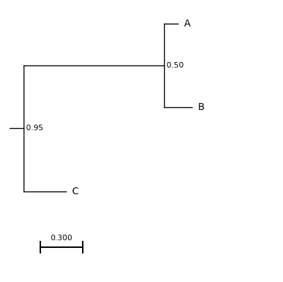
e.g. A string containing a newick formatted tree

# Store the newick data as a string
tree = "((A:0.1,B:0.2)0.5,C:0.3)0.95:0.1;"

# Generate a matplotlib figure
f = plt.figure(figsize=(5, 5))

# Add an axis
ax = plt.subplot()

# Set the axis limits
ax.set_xlim(-1, 15)
ax.set_ylim(-5, 11)

# Visualise the tree
results = plot_phylo.plot_phylo(tree, ax)

# Save the image
f.savefig("examples/from_string.png", bbox_inches='tight')

from_string

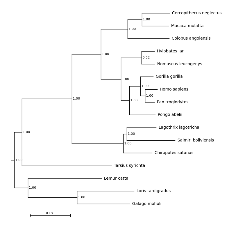
A file containing a newick formatted tree, such as primates.nw.

# Generate a matplotlib figure
f = plt.figure(figsize=(8, 10))

# Add an axis
ax = plt.subplot()

# Plot the tree on this axis, `examples/primates.nw` is the path to the tree
results = plot_phylo.plot_phylo("examples/primates.nw", ax)

# Save the image
plt.savefig("examples/basic_plot.png", bbox_inches='tight')

Basic Tree

`ax`¶

(matplotlib.axes._axes.Axes, Required)

An open matplotlib ax object where the tree will be plotted. Required.

To generate a basic plot with a single subplot:

import matplotlib.pyplot as plt

# Make an empty figure
my_figure = plt.figure()

# Add an empty subplot
my_subplot = my_figure.add_subplot(111)

The object my_subplot is then passed to plot phylo and the tree will be plotted onto this axis.

results = plot_phylo.plot_phylo("examples/primates.nw", my_subplot)

More details about using matplotlib via this object oriented interface are available here.

The advantage of this approach is that you can continue to add features to this plot directly using matplotlib or incorporate your phylogeny into an existing plot.

Positioning the Plot¶

Using the xpos, ypos, height and width parameters, the exact location of the tree within the axis can be specified.

xpos defines the position of the most ancestral node in the tree on the x-axis, excluding the root. In the example tree, this is the split between the bottom three species (lemur, loris and galago) and the remaining primates.

ypos defines the position of the bottom branch of the tree, on the y-axis. In the example tree, this is the branch leading to Galago moholi.

width defines the width of the tree, excluding tip labels, in x-axis units. A tree with a width of 10 and and xpos of 5 will span from positions 5 to 15 on the x axis.

height defines the height of the tree, excluding tip labels, in y-axis units. A tree with a height of 10 and and ypos of 5 will span from positions 5 to 15 on the y axis.

For example:

# Draw the plot and set the axis limits
f = plt.figure(figsize=(8, 10))
ax = plt.subplot()
ax.set_xlim(0, 60)
ax.set_ylim(0, 20)

# Set values for xpos, ypos, height and width
xpos_val = 25
ypos_val = 10
height_val = 5
width_val = 20

# Run the plot_phylo function with these values
results = plot_phylo.plot_phylo("examples/primates.nw", ax, xpos=xpos_val, ypos=ypos_val, height=height_val, width=width_val, show_axis=True, branch_lengths=False, auto_ax=False)

# Annotate these points on the tree using matplotlib functions
# Mark the bottom left corner
ax.scatter(xpos_val, ypos_val, color='red', zorder=2)

# Bottom right corner
ax.scatter(xpos_val + width_val, ypos_val, color='blue', zorder=2)

# Top left corner
ax.scatter(xpos_val, ypos_val+height_val, color='green', zorder=2)

# Top right corner
ax.scatter(xpos_val+width_val, ypos_val+height_val, color='orange', zorder=2)

# Draw a box around this region
ax.plot([xpos_val,
         xpos_val+width_val,
         xpos_val+width_val,
         xpos_val,
         xpos_val],
        [ypos_val,
         ypos_val,
         ypos_val+height_val,
         ypos_val+height_val,
         ypos_val], color='lightgrey', zorder=1)

plt.savefig("examples/tree_pos.png", bbox_inches='tight')

Position

`xpos`¶

(float, Default 0)

Desired position of the root of the tree on the x axis, in axis units.

`ypos`¶

(float, Default 0)

Desired position of the bottom of the tree on the y axis, in axis units.

`height`¶

(float, Default 10) Desired height of the tree, in axis units. Regardless of the height of the axis, the tree with span from ypos to ypos + height.

`width`¶

(float, Default 10) Desired width of the tree, in axis units. Default 10.

`auto-ax`¶

(bool, Default True)

If True, axis limits are determined automatically to best visualise the tree. If False, the user should determine the axis limits directly using matplotlib functionality. Axis limits can still be adjusted later if auto_ax is True.

Visualisation Options¶

`show_axis`¶

(bool, Default False)

Show the axis lines and ticks on the output tree.

`show_support`¶

(bool, Default False)

Display branch support on the internal nodes of the tree.

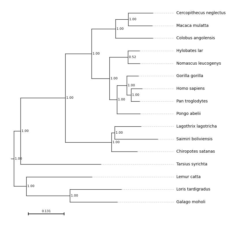
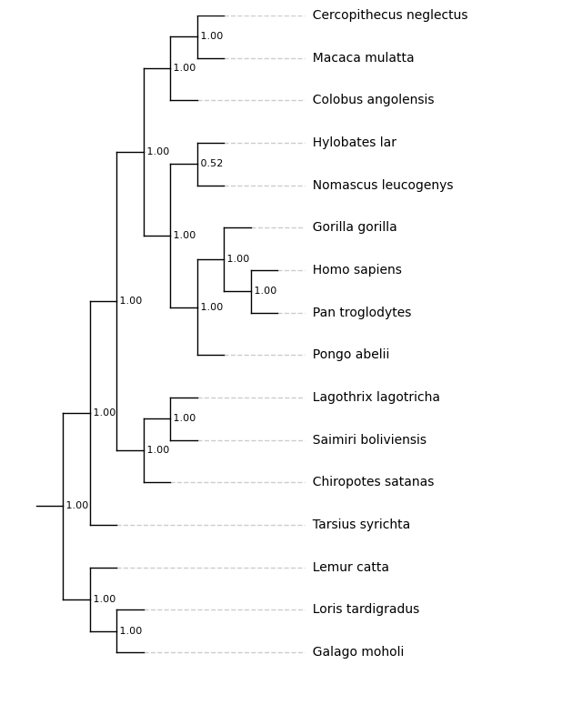
`align_tips`¶

(bool, Default False)

If True, the tip labels will be horizontally aligned rather than positioned at the tips of the branches. By default, they are left-aligned for a standard tree and right-aligned for a mirrored tree (reverse=True)

With align_tips=True

f = plt.figure(figsize=(8, 10))
ax = plt.subplot()
results = plot_phylo.plot_phylo("examples/primates.nw", ax, align_tips=True)
plt.savefig("examples/align_tips.png", bbox_inches='tight')

Aligned Tip Labels

`rev_align_tips`¶

(bool, Default False)

If True the tip labels are right-aligned if reverse=False and left-aligned if reverse=True.

With rev_align_tips=True

f = plt.figure(figsize=(8, 10))
ax = plt.subplot()

# For reverse aligned tip labels the axis limits need to be specified in advance
ax.set_xlim(-1, 12)

results = plot_phylo.plot_phylo("examples/primates.nw", ax, rev_align_tips=True)
plt.savefig("examples/rev_align_tips.png", bbox_inches='tight')

Reverse Aligned Tip Labels

`branch_lengths`¶

(bool, Default True)

If True, the branch lengths provided in the tree are used, otherwise all branches are fixed to the same length. The align tips function can be used in the same way regardless of whether branch lengths are used.

With branch_lengths=False:

f = plt.figure(figsize=(8, 10))

ax = plt.subplot()
ax.set_xlim(-1, 20)
# ylim is set explicitly before drawing the plot
ax.set_ylim(-1, 10)

results = plot_phylo.plot_phylo("examples/primates.nw", ax, branch_lengths=False)

# Save the tree - matplotlib
plt.savefig("examples/nobranchlengths.png", bbox_inches='tight')

No branch lengths

With branch_lengths=False and align_tips=True:

f = plt.figure(figsize=(8, 10))

ax = plt.subplot()
ax.set_xlim(-1, 20)
# ylim is set explicitly before drawing the plot
ax.set_ylim(-1, 10)

results = plot_phylo.plot_phylo("examples/primates.nw", ax, branch_lengths=False, align_tips=True)

# Save the tree - matplotlib
plt.savefig("examples/nobranchlengths_ali.png", bbox_inches='tight')

No branch lengths aligned

`scale_bar`¶

(bool, Default True)

If True and branch_lengths is True, draw a scale bar.

`scale_bar_width`¶

(float, Default None)

Width of scale bar in axis units. If not specified, the scale bar will be 1/4 of the width of the tree.

`reverse`¶

(bool, Default False) * If True, mirror the tree on the y-axis, showing the root on the right-hand side.

With reverse=True:

f = plt.figure(figsize=(8, 10))
ax = plt.subplot()
results = plot_phylo.plot_phylo("examples/primates.nw", ax, reverse=True)
plt.savefig("examples/reversed.png", bbox_inches='tight')

Mirrored Tree

`outgroup`¶

(str, Default None)

Specifies a leaf to set as the outgroup, must be identical to the name in the tree file.

`col_dict`¶

(dict, Default {})

User provided dictionary with tip labels as keys and colours (in any format accepted by matplotlib as values. If this is not specified all labels will be black, if only some labels are specified all others will be black.

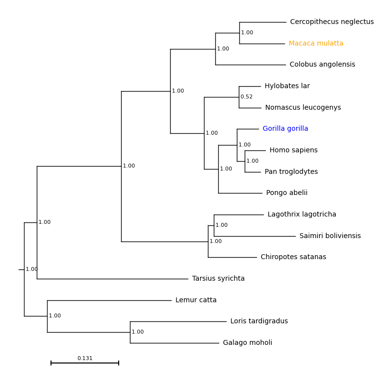
With col_dict={'Macaca mulatta': 'orange, 'Gorilla gorilla': 'blue'}:

f = plt.figure(figsize=(8, 10))
ax = plt.subplot()
results = plot_phylo.plot_phylo("examples/primates.nw", ax, col_dict={'Macaca mulatta': 'orange', 'Gorilla gorilla': 'blue'})
plt.savefig("examples/colours.png", bbox_inches='tight')

Coloured tip labels

`label_dict`¶

(dict, Default {})

User provided dictionary with current tip labels as keys and desired tip labels as values. If this is not specified all labels will be as specified in the newick, if some labels are specified all others will match the newick.

With label_dict={'Macaca mulatta': 'Rhesus macaque, 'Homo sapiens': 'human'}:

f = plt.figure(figsize=(8, 10))
ax = plt.subplot()
results = plot_phylo.plot_phylo("examples/primates.nw", ax, label_dict={'Macaca mulatta': 'Rhesus macaque', 'Homo sapiens': 'human'},
col_dict={'Macaca mulatta': 'orange', 'Homo sapiens': 'blue'})
plt.savefig("examples/labels.png", bbox_inches='tight')

Renamed tips

`font_size`¶

(int, Default 10)

Font size for tip labels. Branch support and scale bar labels will be two sizes smaller.

`line_col`¶

(str or tuple, Default ‘black’)

Line colour, in any format accepted by matplotlib.

`line_width`¶

(float, Default 2)

Line width.

`bold`¶

(list, Default [])

A list of sequence names to show in bold. If sequences are renamed using label_dict, provide the original names.

With bold=['Homo sapiens']:

f = plt.figure(figsize=(8, 10))
ax = plt.subplot()
results = plot_phylo.plot_phylo("%s/examples/primates.nw" % path, ax, bold=['Homo sapiens'])
plt.savefig("examples/bold.png", bbox_inches='tight')

Bold

`collapse`¶

(list, Default [])

`collapse_names`¶

(list, Default [])

Two parameters - collapse and collapse_names are used to allow monophyletic groups to be collapsed, if all tip labels within that clade contain a specific string. The parameter collapse should be a list of strings to look for e.g. ['Saimiri', 'Callithrix']

The parameter collapse_names is a list, in the same order, of the new names to give to the collapsed groups, e.g. ['Saimiri species', 'Callithrix species'].

With the default settings plus outgroup='Lemur_catta'

f = plt.figure(figsize=(10, 8))
ax = f.add_subplot()
plot_phylo.plot_phylo("%s/examples/big_tree_collapse.nw" % path, ax, outgroup='Lemur_catta')
plt.savefig("examples/collapse_before.png", dpi=300)

With collapse=['Eulemur', 'Hapalemur'], collapse_names=['Hapalemur species', 'Eulemur species'], outgroup='Lemur_catta'

f = plt.figure(figsize=(10, 8))
ax = f.add_subplot()
plot_phylo.plot_phylo("%s/examples/big_tree_collapse.nw" % path, ax,
                        outgroup='Lemur_catta',
                        collapse=['Eulemur', 'Hapalemur'],
                        collapse_names=['Eulemur species', 'Hapalemur species'])
plt.savefig("examples/collapse_after.png", dpi=300)

Usage and Parameters¶

Required¶

tree¶

ax¶

Positioning the Plot¶

xpos¶

ypos¶

height¶

width¶

auto-ax¶

Visualisation Options¶

show_axis¶

show_support¶

align_tips¶

rev_align_tips¶

branch_lengths¶

scale_bar¶

scale_bar_width¶

reverse¶

outgroup¶

col_dict¶

label_dict¶

font_size¶

line_col¶

line_width¶

bold¶

collapse¶

collapse_names¶

`tree`¶

`ax`¶

`xpos`¶

`ypos`¶

`height`¶

`width`¶

`auto-ax`¶

`show_axis`¶

`show_support`¶

`align_tips`¶

`rev_align_tips`¶

`branch_lengths`¶

`scale_bar`¶

`scale_bar_width`¶

`reverse`¶

`outgroup`¶

`col_dict`¶

`label_dict`¶

`font_size`¶

`line_col`¶

`line_width`¶

`bold`¶

`collapse`¶

`collapse_names`¶